

How To Create A Pareto Chart In Google Sheets
How to create simple Pareto chart in Excel?
A Pareto chart is composed of a column chart and a line graph, it is used to analyze the quality problems and determine the major factor in the production of quality problems. If you want to create a Pareto chart in your worksheet to display the most common reasons for failure, customer complaints or product defects, I can introduce the steps for you.
- Create a pareto chart in Excel 2016, 2019, or 365
- Create a Pareto chart in Excel 2013 or earlier versions
Create a pareto chart in Excel 2016, 2019, or 365
If you are using Excel 2016, 2019, or 365, you can easily create a pareto chart as follows:
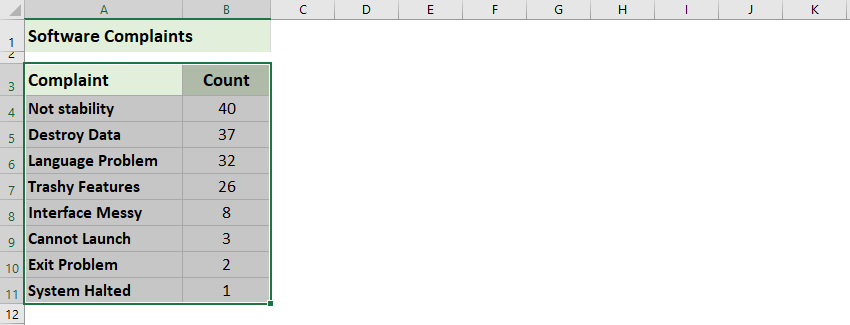
1. Prepare the source data in Excel, and select the source data.
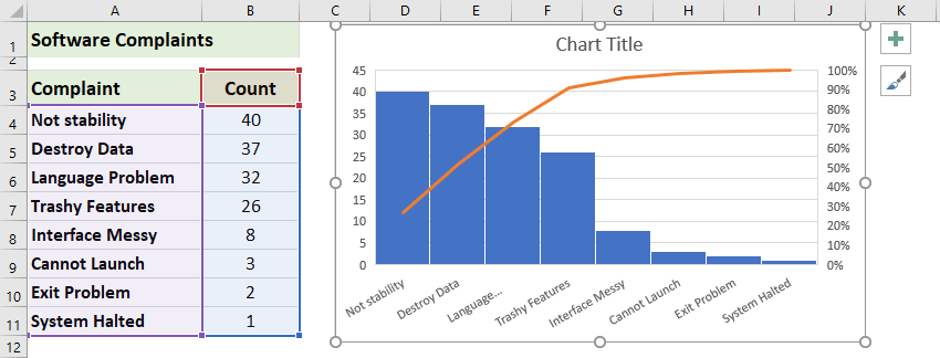
2. Click Insert > Insert Statistic Chart > Pareto.
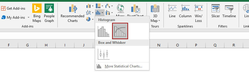
Then the pareto chart is created. See screenshot:
One click to add a cumulative sum line and labels for a cluster column chart
The cluster column chart is quite common and useful in statistic works. Now, Kutools for Excel releases a chart tool – Add Cumulative Sum to Chart to quickly add a cumulative total line and all cumulative total labels for a cluster column chart by only one click! Full Feature Free Trial 30-day!
Kutools for Excel - Includes more than 300 handy tools for Excel. Full feature free trial 30-day, no credit card required! Get It Now
Create a Pareto chart in Excel 2013 or earlier versions
To create a Pareto chart in Excel 2013 or earlier versions, please do as this:
1. Type and list the number of each complaints or defects of your production in a worksheet like the following screenshot:

2. Sort this data in descending order by selecting the cell B4 in this case and clicking Data > Sort Largest to Smallest icon.

And now your values in column B are in descending order as below screenshot shown:

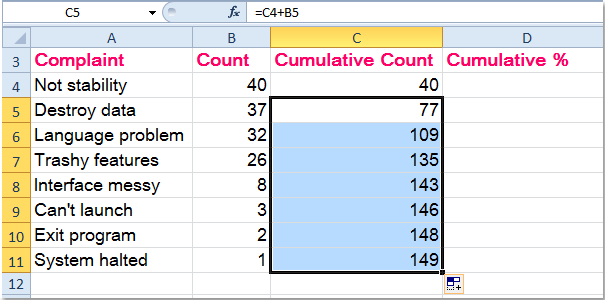
3. Then calculate the Cumulative Count by entering this formula =B4 into the cell C4 in this case, and press Enter key.

4. In cell C5, type this formula =C4+B5 , press Enter key, and select cell C5 then drag the fill handle to the range that you want to contain this formula, and all the Cumulative Count values in column C have been calculated. See screenshots:

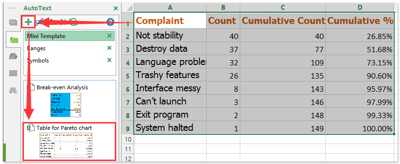
5. Next, you need to calculate the Cumulative Percentage, in cell D4 for example, input this formula =C4/$C$11 , (the cell C4 indicates the number of the first complaints, and the cell C11 contains the total number of the complaints) and then drag the formula down to fill the range you want to use.


Tip: You can format the cell to percentage formatting by selecting the range and right clicking to select Format cells > Percentage.
Tip: Save a range as AutoText entry (remaining cell formats and formulas) for reusing in future
It must be very tedious to refer cells and apply formulas for calculating every time. Kutools for Excel provides a cute workaround of AutoText utility to to save the range as an AutoText entry, which can remain the cell formats and formulas in the range. And then you can reuse this range with just one click in any workbook.
6. And now your data is complete and ready to create a Pareto chart, hold down the Ctrl key select data in column A, column B and column D, and then click Insert > Column > Clustered Column, see screenshot:

7. And you will get a chart as follows:

8. Then select one red bar (Cumulative Percentage) and right click, then choose Change Series Chart Type from the context menu, see screenshot:

9. In the Change Chart Type dialog, select Line with Makers, and click OK. And you will get the chart like the following screenshots shown:


10. And then select the red line, right click and choose Format Data Series, in the Format Data Series dialog box, select Series Options and check Secondary Axis in the right section. See screenshots:


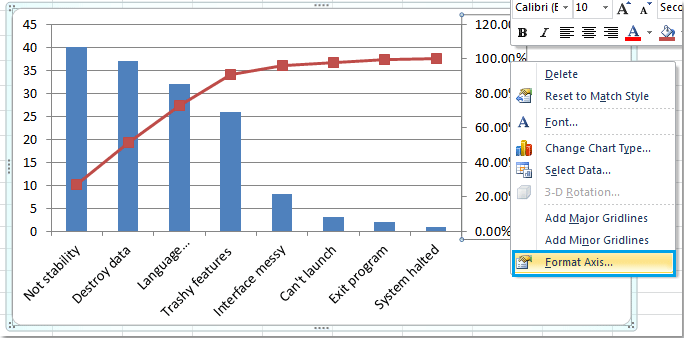
11. Then close the dialog, and the secondary axis has been added to the chart, go on selecting the percentage axis and right clicking to choose Format Axis.
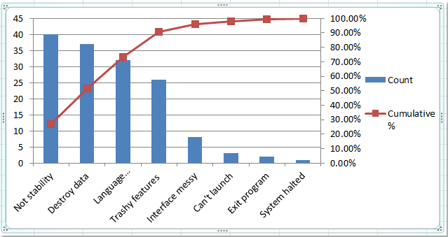
12. In the Format Axis dialog, check Fixed radio button beside Maximum, and set the number to 1.0 in to the text box. See screenshot:

13. And then close the dialog, the Pareto chart has been finished completely as following screenshot:
Demo: Create a simple Pareto chart in Excel
Kutools for Excel includes more than 300 handy tools for Excel, free to try without limitation in 30 days. Download and Free Trial Now!
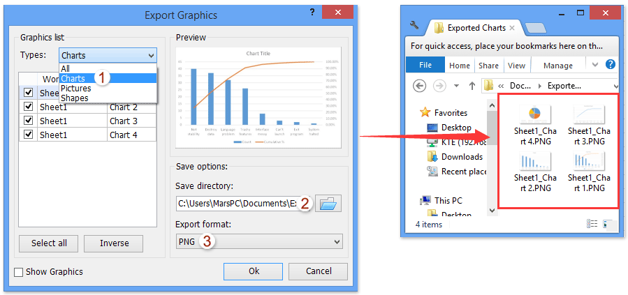
Apply Kutools for Excel's Export Graphics utility to quickly export all charts as images
You can apply Kutools for Excel's Export Graphics utility to quickly export all shapes, charts, pictures, word arts in current workbook to PNG/JPG/TIF/GIF images with ease. Full Feature Free Trial 30-day!
Related articles:
The Best Office Productivity Tools
Kutools for Excel Solves Most of Your Problems, and Increases Your Productivity by 80%
- Reuse: Quickly insert complex formulas, charts and anything that you have used before; Encrypt Cells with password; Create Mailing List and send emails...
- Super Formula Bar (easily edit multiple lines of text and formula); Reading Layout (easily read and edit large numbers of cells); Paste to Filtered Range...
- Merge Cells/Rows/Columns without losing Data; Split Cells Content; Combine Duplicate Rows/Columns... Prevent Duplicate Cells; Compare Ranges...
- Select Duplicate or Unique Rows; Select Blank Rows (all cells are empty); Super Find and Fuzzy Find in Many Workbooks; Random Select...
- Exact Copy Multiple Cells without changing formula reference; Auto Create References to Multiple Sheets; Insert Bullets, Check Boxes and more...
- Extract Text, Add Text, Remove by Position, Remove Space; Create and Print Paging Subtotals; Convert Between Cells Content and Comments...
- Super Filter (save and apply filter schemes to other sheets); Advanced Sort by month/week/day, frequency and more; Special Filter by bold, italic...
- Combine Workbooks and WorkSheets; Merge Tables based on key columns; Split Data into Multiple Sheets; Batch Convert xls, xlsx and PDF...
- More than 300 powerful features. Supports Office/Excel 2007-2019 and 365. Supports all languages. Easy deploying in your enterprise or organization. Full features 30-day free trial. 60-day money back guarantee.
")
Office Tab Brings Tabbed interface to Office, and Make Your Work Much Easier
- Enable tabbed editing and reading in Word, Excel, PowerPoint , Publisher, Access, Visio and Project.
- Open and create multiple documents in new tabs of the same window, rather than in new windows.
- Increases your productivity by 50%, and reduces hundreds of mouse clicks for you every day!
")
How To Create A Pareto Chart In Google Sheets
Source: https://www.extendoffice.com/documents/excel/1443-excel-create-pareto-chart.html
Posted by: shustermuder1970.blogspot.com
0 Response to "How To Create A Pareto Chart In Google Sheets"
Post a Comment